Quadratic Equations with Complex Roots

R Packages

library(tidyverse)
library(ggformula)
library(mosaic)

Quadratic Roots and Equations Family

quad_eq <- function(a, b, c, x) {
  a*x^2 + b*x + c
}

parabola <- function(a,x){a*x^2}
line <- function(b,c, x){-b*x - c}
discrim <- function(a,b,c){b^2 - 4*a*c}
roots <- function(a,b,c, discrim){
  dplyr::if_else(discrim >= 0, 
            tibble(Re1 = (-b + sqrt(discrim))/(2*a), 
                         Im1 = 0,
                         Re2 = (-b -sqrt(discrim))/(2*a),
                         Im2 = 0), 
            
            tibble(Re1 = -b/(2*a),
                          Im1 = sqrt(abs(discrim))/(2*a), 
                          Re2 = -b/(2*a),
                          Im2 = -sqrt(abs(discrim))/(2*a))
                   )
}

## Roots Graph Function

root_graph <- function(a,b,c){
  p <- expand_grid(tibble(a,b,c,
                     x = list(seq(from = -5, to = 5, 
                                  by = 0.1)))) %>% 
  
  dplyr::mutate(discrim = discrim(a,b,c)) %>%
  
  dplyr::mutate(geoms = purrr::pmap(
    .l = list(a,b,c, x),
    .f = \(a,b,c, x) tibble(x = x, 
                            curve_eq = parabola(a,x), 
                            line_eq = line(b,c,x),
                            quad_eq = quad_eq(a,b,c,x)))) %>%
          
  dplyr::mutate(roots = purrr::pmap(
    .l = list(a,b,c, discrim),
    .f = \(a,b,c, discrim) roots(a,b,c, discrim))) %>% 
  
    unnest(roots) %>% 
    select(a,b,c, discrim, Re1, Im1, Re2, Im2) %>%
    mutate(sign = dplyr::if_else(discrim < 0, "Complex", "Real")) %>% 
  gf_point(Im1 ~ Re1, color = ~ sign) %>% 
  gf_point(Im2 ~ Re2, color = ~ sign) %>% 
  gf_labs(title = "Roots of Quadratic Equations",
          subtitle = "",
          x = "Real Part",
          y = "Imaginary Part") %>%
  # gf_text(label = ~discrim, nudge_y = 0.25) %>%
  gf_refine(coord_cartesian(), theme_classic())
  
  return(p)
}

Let us set up a data frame containing several values for a, b, and c.

quad_data <- expand_grid(
  a = c(-5, -3, -1, 1, 3, 5),
  c = c(-5, -3, -1, 1, 3, 5),
  b = c(-5, -3, -1, 1, 3, 5),
  x = list(seq(from = -5, to = 5, by = 0.1)))

my_charts <- quad_data %>% 
  
  dplyr::mutate(discrim = discrim(a,b,c)) %>%
  
  dplyr::mutate(geoms = purrr::pmap(
    .l = list(a,b,c, x),
    .f = \(a,b,c, x) tibble(x = x, 
                            curve_eq = parabola(a,x), 
                            line_eq = line(b,c,x),
                            quad_eq = quad_eq(a,b,c,x)))) %>%
  
  # dplyr::mutate(graphs = pmap(
  #   .l = list(geoms),
  #   .f = \(geoms) (ggplot() +
  #       geom_line(aes(x = x, y = curve_eq), data = geoms) +
  #       geom_line(aes(x = x, y = line_eq), data = geoms, color = "red") + theme_minimal()))) %>% 
          
  dplyr::mutate(roots = purrr::pmap(
    .l = list(a,b,c, discrim),
    .f = \(a,b,c, discrim) roots(a,b,c, discrim)))
    
# for(i in 1:nrow(my_charts)) {
#   print(my_charts$graphs[[i]])
# }

my_charts_selected <- my_charts %>% 
  unnest(roots) %>% 
  select(a,b,c, discrim, Re1, Im1, Re2, Im2) %>%
  mutate(sign = dplyr::if_else(discrim < 0, "Complex", "Real")) 
my_charts_selected

ABCDEFGHIJ0123456789

a <dbl>	b <dbl>	c <dbl>	discrim <dbl>	Re1 <dbl>	Im1 <dbl>	Re2 <dbl>	Im2 <dbl>	sign <chr>
-5	-5	-5	-75	-0.5000000	-0.8660254	-0.5000000	0.8660254	Complex
-5	-3	-5	-91	-0.3000000	-0.9539392	-0.3000000	0.9539392	Complex
-5	-1	-5	-99	-0.1000000	-0.9949874	-0.1000000	0.9949874	Complex
-5	1	-5	-99	0.1000000	-0.9949874	0.1000000	0.9949874	Complex
-5	3	-5	-91	0.3000000	-0.9539392	0.3000000	0.9539392	Complex
-5	5	-5	-75	0.5000000	-0.8660254	0.5000000	0.8660254	Complex
-5	-5	-3	-35	-0.5000000	-0.5916080	-0.5000000	0.5916080	Complex
-5	-3	-3	-51	-0.3000000	-0.7141428	-0.3000000	0.7141428	Complex
-5	-1	-3	-59	-0.1000000	-0.7681146	-0.1000000	0.7681146	Complex
-5	1	-3	-59	0.1000000	-0.7681146	0.1000000	0.7681146	Complex

Next

123456

...

22

Previous

1-10 of 216 rows

my_charts_selected %>% 
  gf_point(Im1 ~ Re1, color = ~ sign) %>% 
  gf_point(Im2 ~ Re2, color = ~ sign) %>% 
  gf_labs(title = "Roots of Quadratic Equations",
          subtitle = "a, b, c all varying",
          x = "Real Part",
          y = "Imaginary Part") %>%
  # gf_text(label = ~discrim, nudge_y = 0.25) %>%
  gf_refine(coord_cartesian(), theme_classic())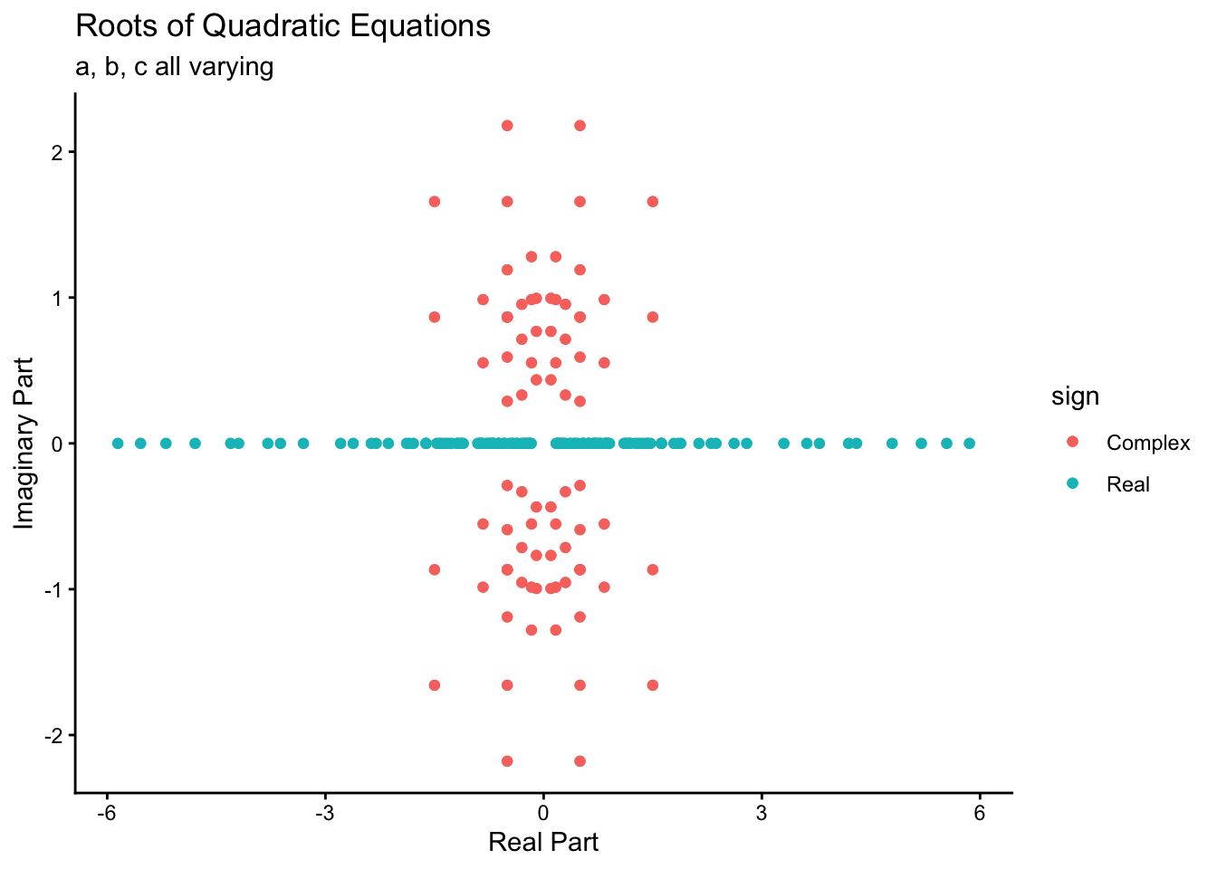

Slope b Constant, c intercept varying

# Slope b = 1
expand_grid(
  a = c(1, 1,1,1,1,1),
  c = c(-5, -3, -1, 1, 3, 5),
  b = c(1, 1,1,1,1,1),
  x = list(seq(from = -5, to = 5, by = 0.1))) %>% 
  
  dplyr::mutate(discrim = discrim(a,b,c)) %>%
  
  dplyr::mutate(geoms = purrr::pmap(
    .l = list(a,b,c, x),
    .f = \(a,b,c, x) tibble(x = x, 
                            curve_eq = parabola(a,x), 
                            line_eq = line(b,c,x),
                            quad_eq = quad_eq(a,b,c,x)))) %>%
  dplyr::mutate(roots = purrr::pmap(
    .l = list(a,b,c, discrim),
    .f = \(a,b,c, discrim) roots(a,b,c, discrim))) %>% 
  unnest(roots) %>% 
  select(a,b,c, discrim, Re1, Im1, Re2, Im2) %>%
  mutate(sign = dplyr::if_else(discrim < 0, "Complex", "Real")) %>% 
  gf_point(Im1 ~ Re1, color = ~ sign) %>% 
  gf_point(Im2 ~ Re2, color = ~ sign) %>% 
  gf_labs(title = "Roots of Quadratic Equations",
          subtitle = "Slope b = 1, Intercept c varying",
          x = "Real Part",
          y = "Imaginary Part") %>%
  # gf_text(label = ~discrim, nudge_y = 0.25) %>%
  gf_refine(coord_cartesian(), theme_classic())
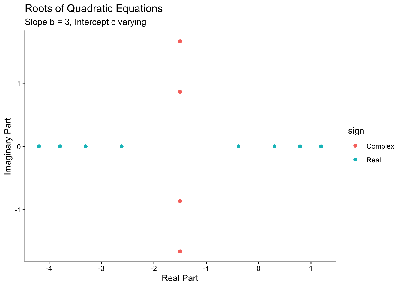
# Slope b = 3
expand_grid(
  a = c(1, 1,1,1,1,1),
  c = c(-5, -3, -1, 1, 3, 5),
  b = 3,
  x = list(seq(from = -5, to = 5, by = 0.1))) %>% 
  
  dplyr::mutate(discrim = discrim(a,b,c)) %>%
  
  dplyr::mutate(geoms = purrr::pmap(
    .l = list(a,b,c, x),
    .f = \(a,b,c, x) tibble(x = x, 
                            curve_eq = parabola(a,x), 
                            line_eq = line(b,c,x),
                            quad_eq = quad_eq(a,b,c,x)))) %>%
  dplyr::mutate(roots = purrr::pmap(
    .l = list(a,b,c, discrim),
    .f = \(a,b,c, discrim) roots(a,b,c, discrim))) %>% 
  unnest(roots) %>% 
  select(a,b,c, discrim, Re1, Im1, Re2, Im2) %>%
  mutate(sign = dplyr::if_else(discrim < 0, "Complex", "Real")) %>% 
  gf_point(Im1 ~ Re1, color = ~ sign) %>% 
  gf_point(Im2 ~ Re2, color = ~ sign) %>% 
  gf_labs(title = "Roots of Quadratic Equations",
          subtitle = "Slope b = 3, Intercept c varying",
          x = "Real Part",
          y = "Imaginary Part") %>%
  # gf_text(label = ~discrim, nudge_y = 0.25) %>%
  gf_refine(coord_cartesian(), theme_classic())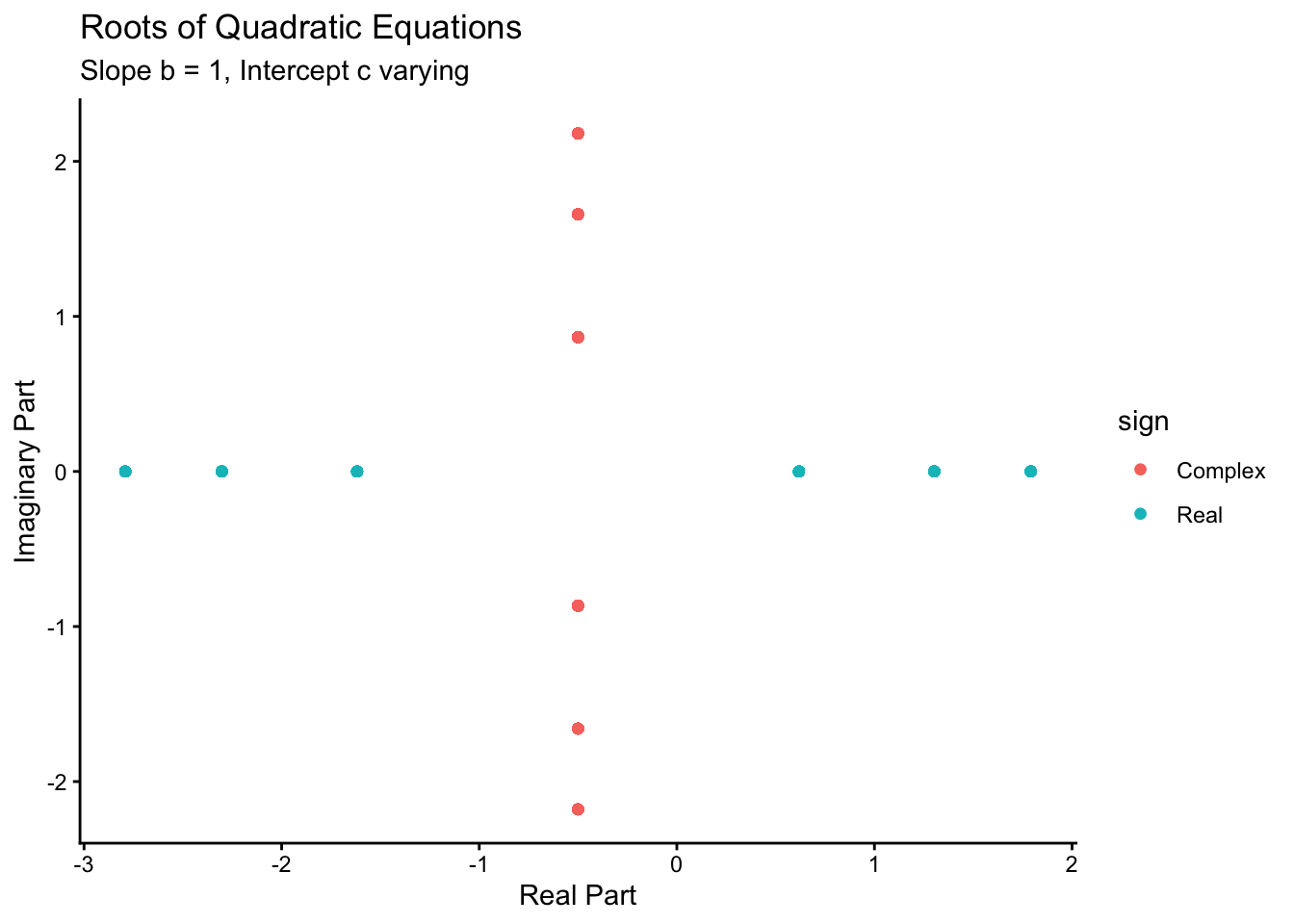

Slope b varying, intercept constant

quad_data <- expand_grid(
  a = c(1, 1,1,1,1,1),
  b = seq(-3, 3, by = 0.25),
  c = c(1, 1,1,1,1,1),
  x = list(seq(from = -5, to = 5, by = 0.1)))

quad_data %>% 
  
  dplyr::mutate(discrim = discrim(a,b,c)) %>%
  
  dplyr::mutate(geoms = purrr::pmap(
    .l = list(a,b,c, x),
    .f = \(a,b,c, x) tibble(x = x, 
                            curve_eq = parabola(a,x), 
                            line_eq = line(b,c,x),
                            quad_eq = quad_eq(a,b,c,x)))) %>%
  dplyr::mutate(roots = purrr::pmap(
    .l = list(a,b,c, discrim),
    .f = \(a,b,c, discrim) roots(a,b,c, discrim))) %>% 
  unnest(roots) %>% 
  select(a,b,c, discrim, Re1, Im1, Re2, Im2) %>%
  mutate(sign = dplyr::if_else(discrim < 0, "Complex", "Real")) %>% 
  gf_point(Im1 ~ Re1, color = ~ sign) %>% 
  gf_point(Im2 ~ Re2, color = ~ sign) %>% 
  gf_labs(title = "Roots of Quadratic Equations",
          x = "Real Part",
          y = "Imaginary Part") %>%
  # gf_text(label = ~discrim, nudge_y = 0.25) %>%
  gf_refine(coord_fixed(), theme_classic())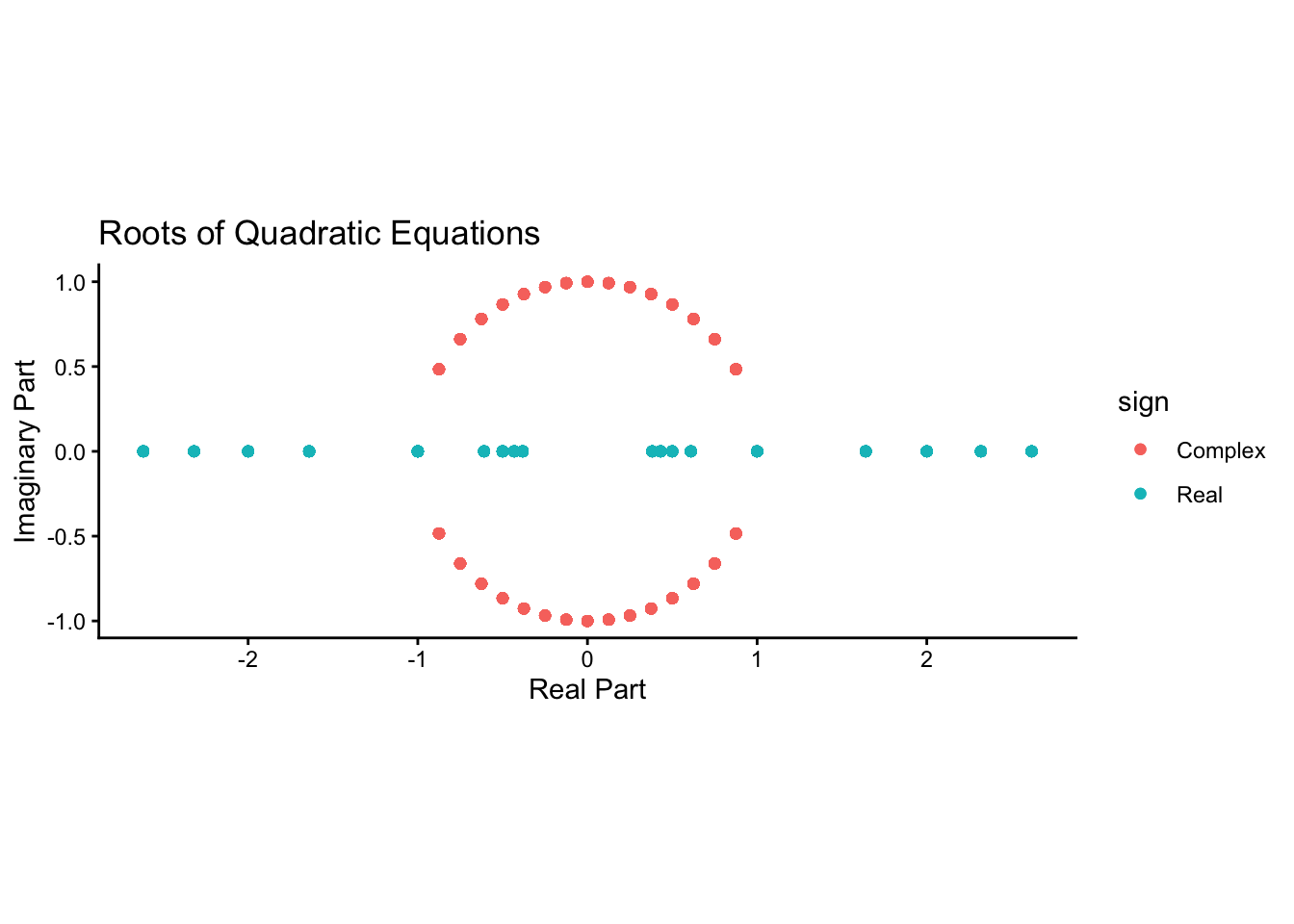

Observations

The roots of the quadratic equation seem to have a similar kind of loci as we saw ( long ago!) with Root Locus plots for control systems. The roots are real initially and converge towards zero (b = 0, c = 0; discriminant = 0) and then diverge into the complex plane as the discriminant becomes negative.

How do I plot this on a 3D plot showing the parabola (y = ax^2) and the line (y = -bx - c) intersecting in the complex plane? and how do I animate the transition from real to complex roots?